Using Geographic Information Systems (GIS) in  and
and  
Geographic Information Systems (GIS)
GIS refers to methods of storing, displaying and analyzing geogaphical information. These methods have become essential in economic analysis (as you have noticed from the reading list for our Ph.D. course on economic growth). For this reason, it is good that you acquaint yourself with these methods. They will prove very useful when doing research, especially to show the spatial distribution of your variables of interest, contructing new measures, or doing spatial analysis.
Software
Commercial
There are various GIS specialized programs and packages. ESRI produces ArcGIS, which is the most known and commonly used commercial software. It is very easy to use to produce maps and do simple computations. Most universities (including ours) offer it in their computer labs. The main disadvantages are that it requires a computer running Windows, it is costly, and extremely slow for computations. Of course this is changing, e.g., now you can use it online.
Nonetheless, I always suggest you use and learn open-source alternatives.
Open Source
There are many open source GIS projects, many of which are supported/gathered at ![]() . The most known and widely used seem to be
. The most known and widely used seem to be ![]() and
and ![]() , although Python is increasingly becoming the language of GIS. QGIS can be programmed in Python and many web-based GIS services and databases are programmed in Python. Furthermore, there are many new Python packages which allow you to import, export, analyze, visualize, etc. GIS data. THis notebook will serve as a basic introduction, which I hope to develop further with time. Many of the solutions provded here have been implemented by myself or taken from sources on the web (regretfully I did not keep track from where I took some ideas or snipplets of code, so I cannot provide due credit).
, although Python is increasingly becoming the language of GIS. QGIS can be programmed in Python and many web-based GIS services and databases are programmed in Python. Furthermore, there are many new Python packages which allow you to import, export, analyze, visualize, etc. GIS data. THis notebook will serve as a basic introduction, which I hope to develop further with time. Many of the solutions provded here have been implemented by myself or taken from sources on the web (regretfully I did not keep track from where I took some ideas or snipplets of code, so I cannot provide due credit).
Installation
Anaconda (Suggested)
If you followed the steps for installing the Continuum Anaconda Python Distribution and for creating the GeoPythonXenv (presented here), then you are basically set for working with GIS in Python + R.
Non Anaconda installation (Discouraged - old and may not work anymore)
Here I will give you the basic idea of what you need to install to have a working GIS environment. I assume you have already installed Canopy with all the pakages provided by Enthought. Additionally, you will need to install GRASS, QGIS, and GDAL/OGR.
Windows
Download the installers in each of these websites and you should be done!
Mac OSX
There are various methods of getting these on your computer.
I used to install using the installers provided by Kyngchaos. But I have moved to using HomeBrew, which allows you install many other GNU projects. To do so, open a terminal window (I recommend getting iTerm2, which is more powerful than the one provided by OSX) and run the following code (I think you will need to have Xcode and its command-line utilities installed)
ruby -e "$(curl -fsSL https://raw.github.com/Homebrew/homebrew/go/install)"
brew doctor
This should install HomeBrew on your system and let you know of any issues. Once you have done so and have a working homebrew installation, you will be able to install packages and programs using the brew install command. Before doing so, you should run the following commands
brew update
brew tap homebrew/science
This will update HomeBrew's formulas to the latest version. Now issue the command
brew cask install qgis
You should be done and have teh latest vanilla version of QGIS in your Applications folder.
Not a vanilla fan?
Ok. sometimes you want QGIS with all the additional blows and whistles, e.g. integration with GRASS, etc. In that case, you need a bit more work. Luckily there are awesome people who are trying to keep this streamlined and working for all of us. Head to osgeo4mac and follow their instructions.
Note on GDAL + Canopy
It seems Canopy already has GDAL incorporated, at least so it seems on Mac OS X. But there is a bug that might prevent it from working, unless you add the following line on your .profile
export GDAL_DATA=~/Library/Enthought/Canopy_64bit/User/share/gdalData
Ok...now that we have a working GIS desktop system, let us talk a little about types of data. All GIS data includes elements with their properties and their geographical information like location, as determined by e.g. latitude and longitude, address, zip code, etc. So, for example an element might be a country, its properties might be GDP per capita, Gini coefficient, etc. and its location. Another example might be a restaurant with its menu and prices, services (dine-in, take-out, delivery), area of service and location.
Formats
GIS comes in very different formats, althogh most of them can be categorizewd into two types Rasters and Vector formats.
- Rasters are basically matrices $R=[R_{ij}]$ of size $m\times n$ that hold numerical information, where each cell $R_{ij}$ shows the value of interest at a specific location $ij$. Where this location $ij$ is, is determined by the actual format and the projection of the data (this will be clearer below).
- Vectors represent a geographical element geometrically and include additional information on it. An element can be represented as one of the following geometries:
- A point or set of unconnected points
- A line or set of (un)connected lines
- A Polygon
- A set of one or various of the previous types
Examples of Raster formats:
- GeoTiff: Multipurpose raster format.
- ESRI Grid: Main ESRI raster format.
- Digital Elevation Model (DEM): Used by the US Geological Survey to record elevation data.
- Band Interleaved by Line, Band Interleaved by Pixel, Band Sequential (BIL, BIP, BSQ): These data formats are typically used by remote sensing systems.
- Digital Raster Graphic (DRG): This format is used to store digital scans of paper maps.
Examples of Vector formats:
- Shapefile: An open specification, developed by ESRI, for storing and exchanging GIS data. A Shapefile actually consists of a collection of files all with the same base name, for example hawaii.shp, hawaii.shx, hawaii.dbf, and so on.
- Simple Features: An OpenGIS standard for storing geographical data (points, lines, polygons) along with associated attributes.
- TIGER/Line: A text-based format previously used by the U.S. Census Bureau to describe geographic features such as roads, buildings, rivers, and coastlines. More recent data comes in the Shapefile format, so the TIGER/Line format is only used for earlier Census Bureau datasets.
- Coverage: Proprietary data format used by ESRI's ARC/INFO system.
Other formats:
- Well-known Text (WKT): text-based format for representing a single geographic feature such as a polygon or line.
- Well-known Binary (WKB): similar to WKT uses binary data rather than text to represent a single geographic feature.
- GeoJSON: An open format for encoding geographic data structures, based on the JSON data interchange format. This is becoming the internet's prefered format.
Sources of Data
There are many places to find data. Some useful links to start are:
- WorldMap
- FAO's GeoNetwork
- IPUMS USA Boundary files for Censuses
- IPUMS International Boundary files for Censuses
- GADM database of Global Administrative Areas
- Global Administrative Unit Layers
- Natural Earth: Various vector and raster files with all kinds of geographical, cultural and socioeconomic variables
- Global Map
- Digital Chart of the World
- Sage and Sage Atlas
- Ramankutti's Datasets on land use, crops, etc.
- SEDAC at Columbia University: Gridded Population, Hazzards, etc.
- World Port Index
- USGS elevation maps
- NOOA's Global Land One-km Base Elevation Project (GLOBE)
- NOOA Nightlight data: This is the data used by Henderson, Storeygard, and Weil AER 2012 paper.
- Other NOOA Data
- GEcon
- OpenStreetMap
- U.S. Census TIGER
- Geo-referencing of Ethnic Groups
See also Wikipedia links
Creating maps and exploring data
Let us start by creating some simple maps. For this, create a directory called mydata in your $HOME directory and download the following datasets and extract them:
- The full GADM shape file is available for download here, since it is large, also download the file for your country of origin from here.
- Natural Earth's Populated Places dataset
- Ramankutty's Suitability Index
- Lights Data for 2012
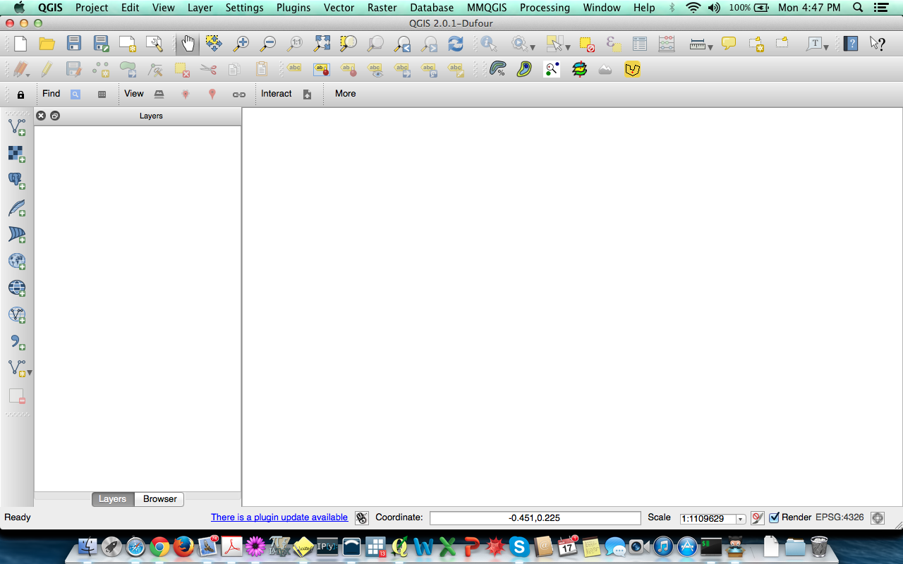
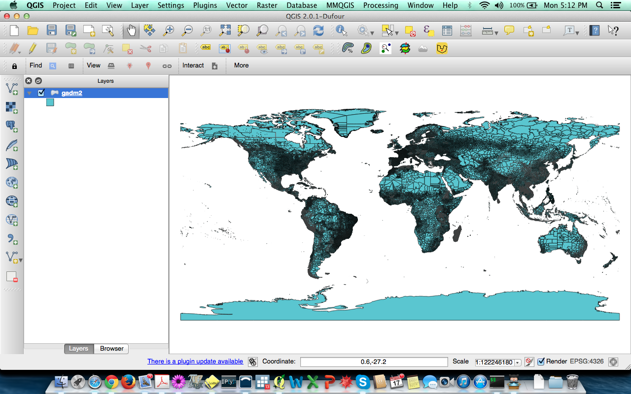
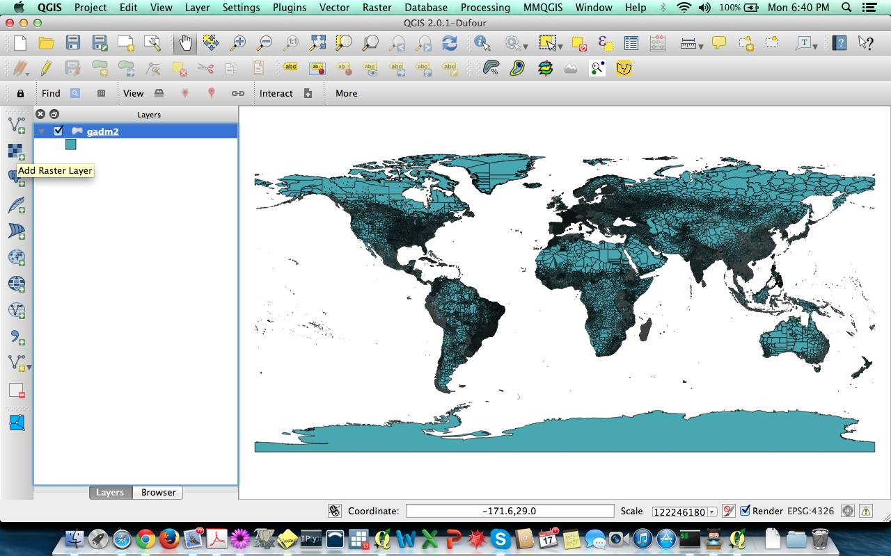
Now, open QGIS. You should see something like this
To open a file in QGIS you can:
- Use
FinderorWindows Explorerto navigate to the file anddouble-clickon it. - Use the
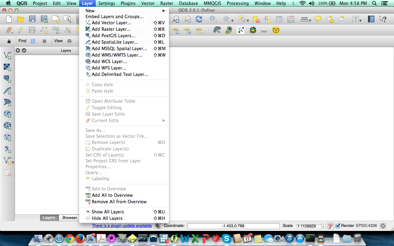
Layermenu in QGIS
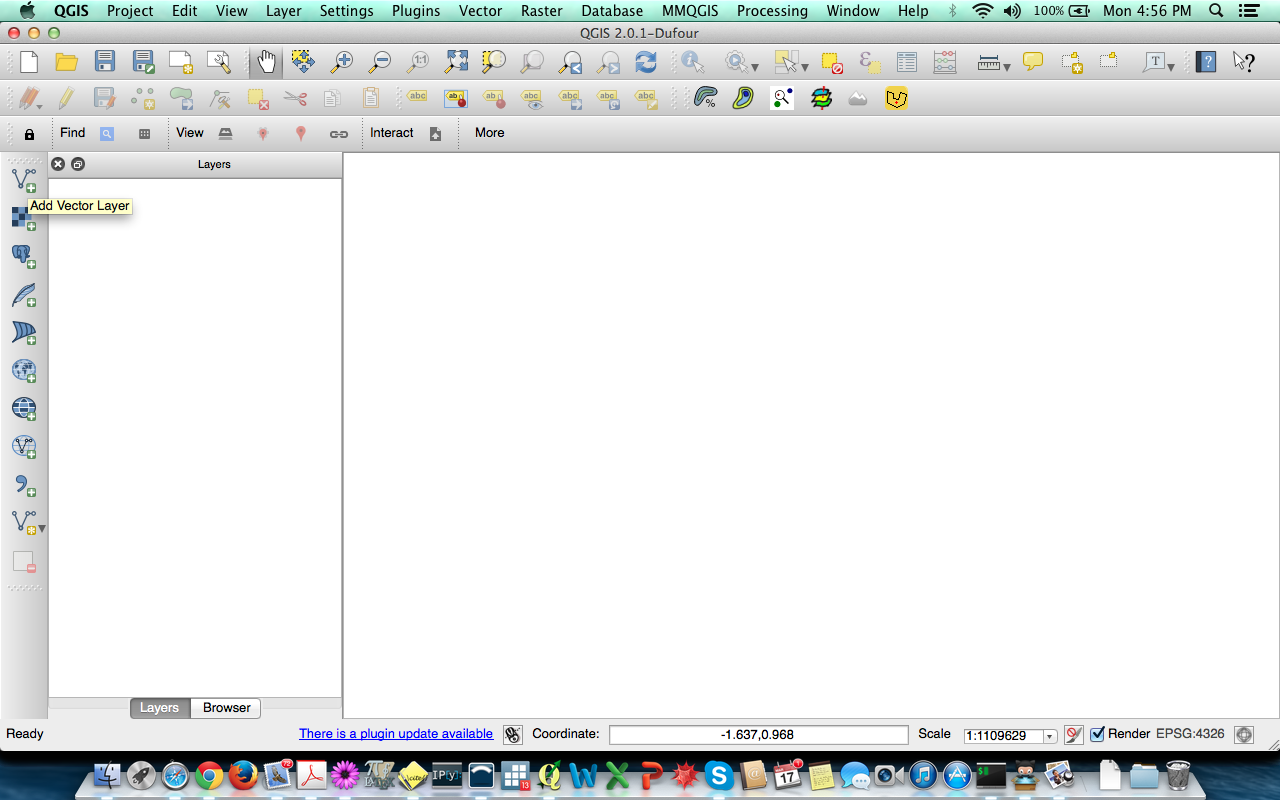
- Use the toolbar on the left

Working with vector layers
Let's start by adding the vector file for your country of origin using the add vector layer button in the toolbar.
I have added the full GADM dataset, so it looks like this
Now we can use various tools available within QGIS to learn about the data, select the data, analyze the data, etc.
The handtool for panning:

- Try it out, use the tool to move your country around the screen.
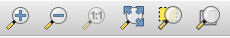
Zoom in/out/to selection/full:
- Try it out, by zooming around your city of birth.
Identify Features:

- Try it out, click on the feature you just zoomed into. Did you zoom into the correct feature?
Select Features:

- Try it out, select the feature of the region where you were born.
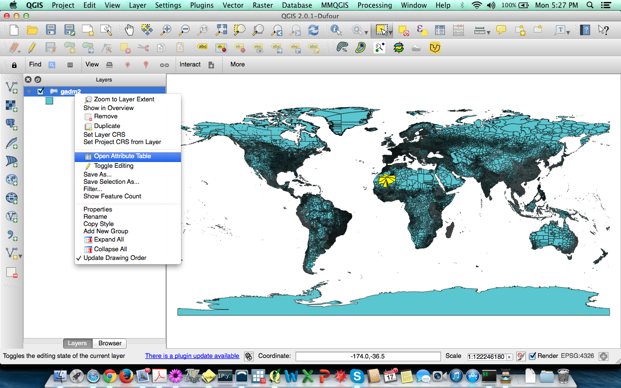
Besides the geometrical information that we observe, most Shape files have other information relating to each feature. This information is contained in the Attribute Table, which can be accessed with
- the
Open Attribute Tablebutton
- By
right-clickingon the name of the layer in the left panel
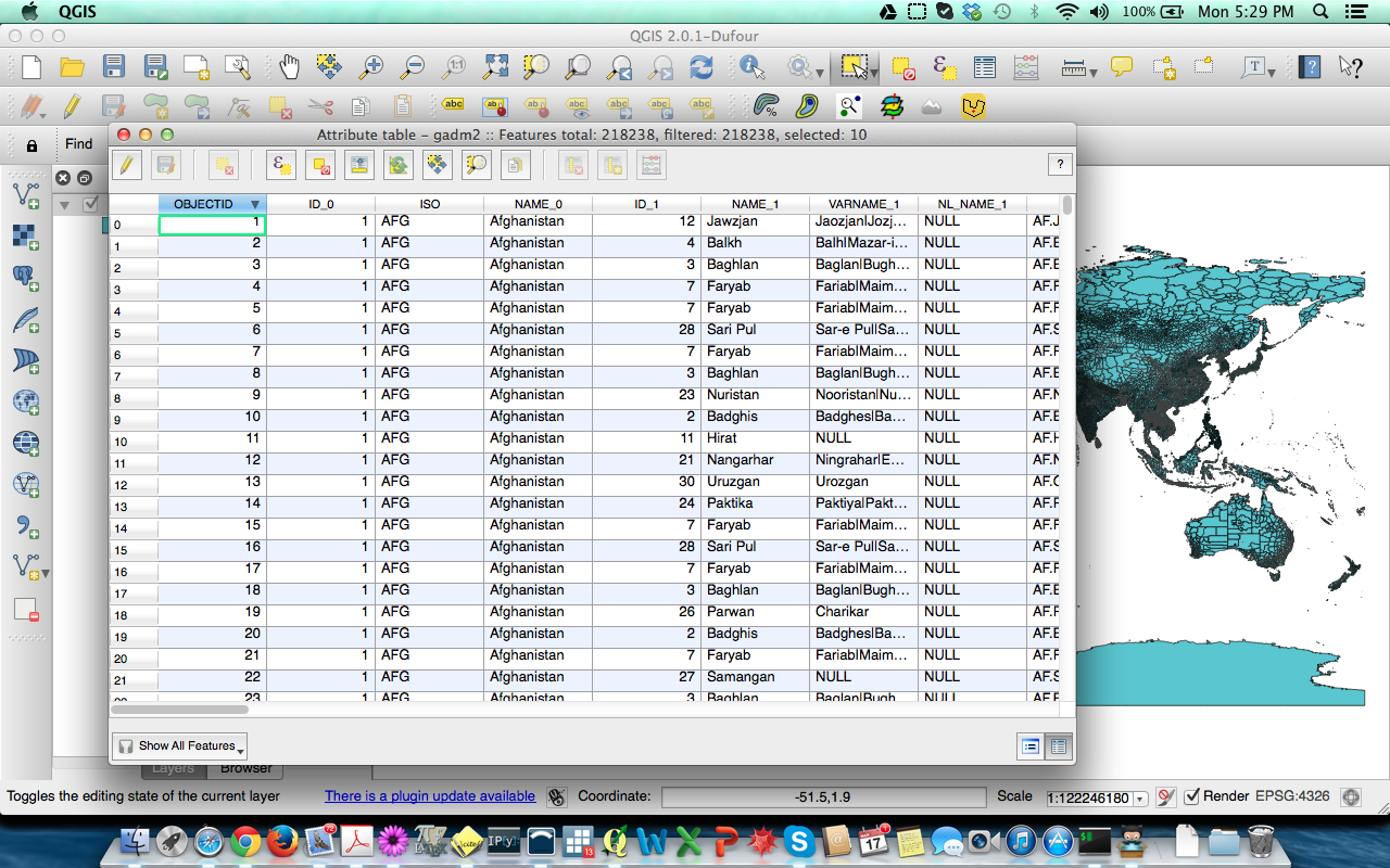
Doing so shows you the additional information contained in the shape file. For the GADM file it includes
- the identification number of the feature
OBJECTID - the identification number of the country (Administrative Level 0) to which the feature belongs
ID_0 - the ISO-3 code of the country to which the feature belongs
ISO - the name of the country to which the feature belongs
NAME_0 - the identification number of the region in the country (Administrative Level 1) to which the feature belongs
ID_1
etc.
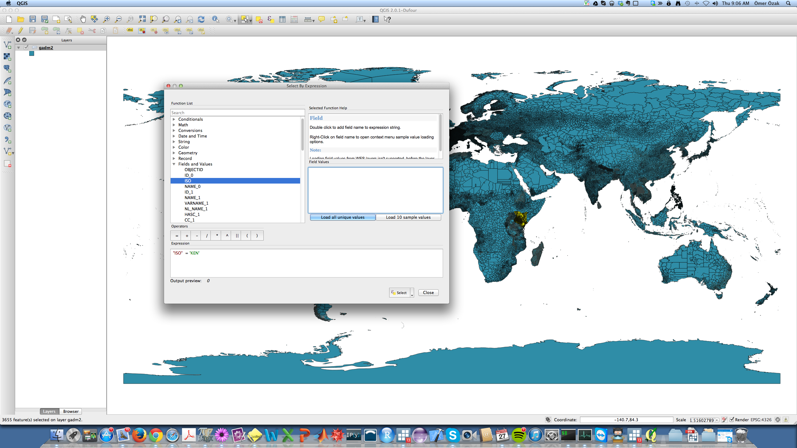
We can use this information to color our maps, or to select features for further analysis. I will use the select feature using an expression button  to select all features which have the ISO-3 code for Kenya. Once you click on the button, you will see the following window, where you can write the expression to be used to select features. In this case I wrote the expression
'ISO'='KEN'
to select all features with Kenya's ISO-3 code.
Sometimes we will want to work with a subset of features, especially if the data we are working has many features, like the GADM data. To select a subset of the features and only work with those, use the Layer->Query option in the Menu as shown below
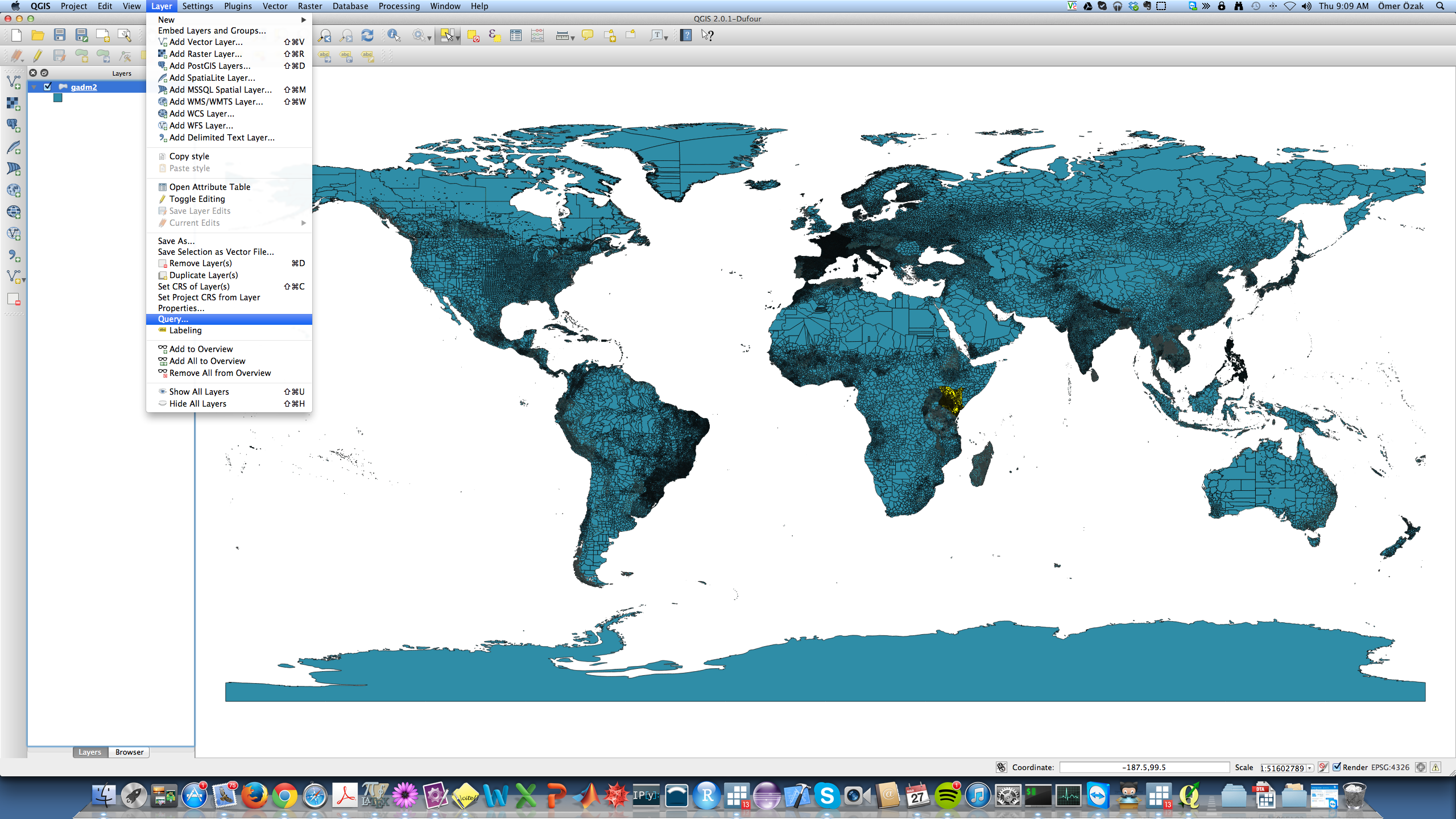
This opens a window where you can write expression as the previous one, to select features by their attributes. These are SQL expressions and have to conform to SQL's grammar (we will not go into this at this point). Once I execute the same expression as above
'ISO'='KEN'
QGIS leaves only the features in Kenya for analysis.
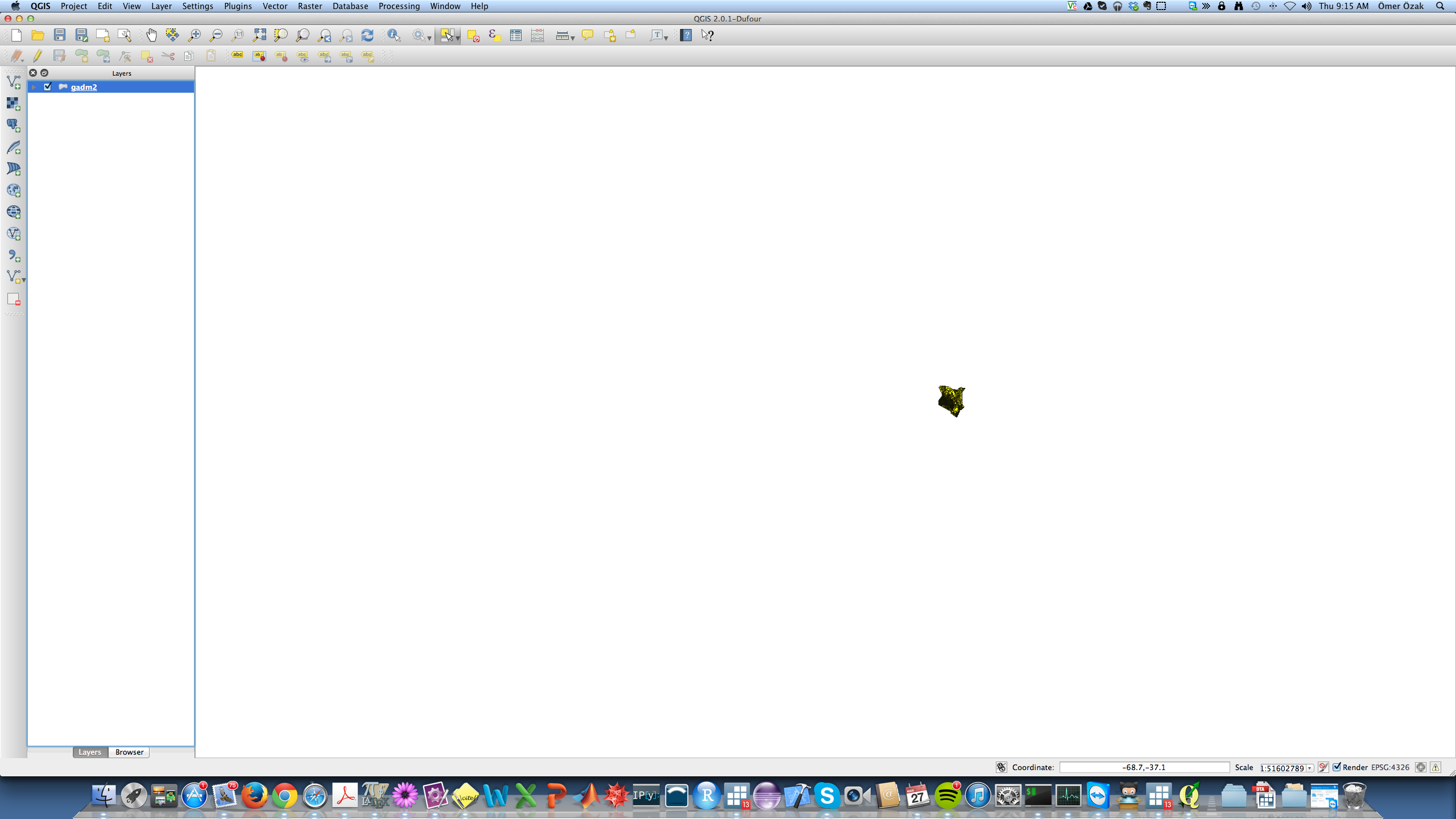
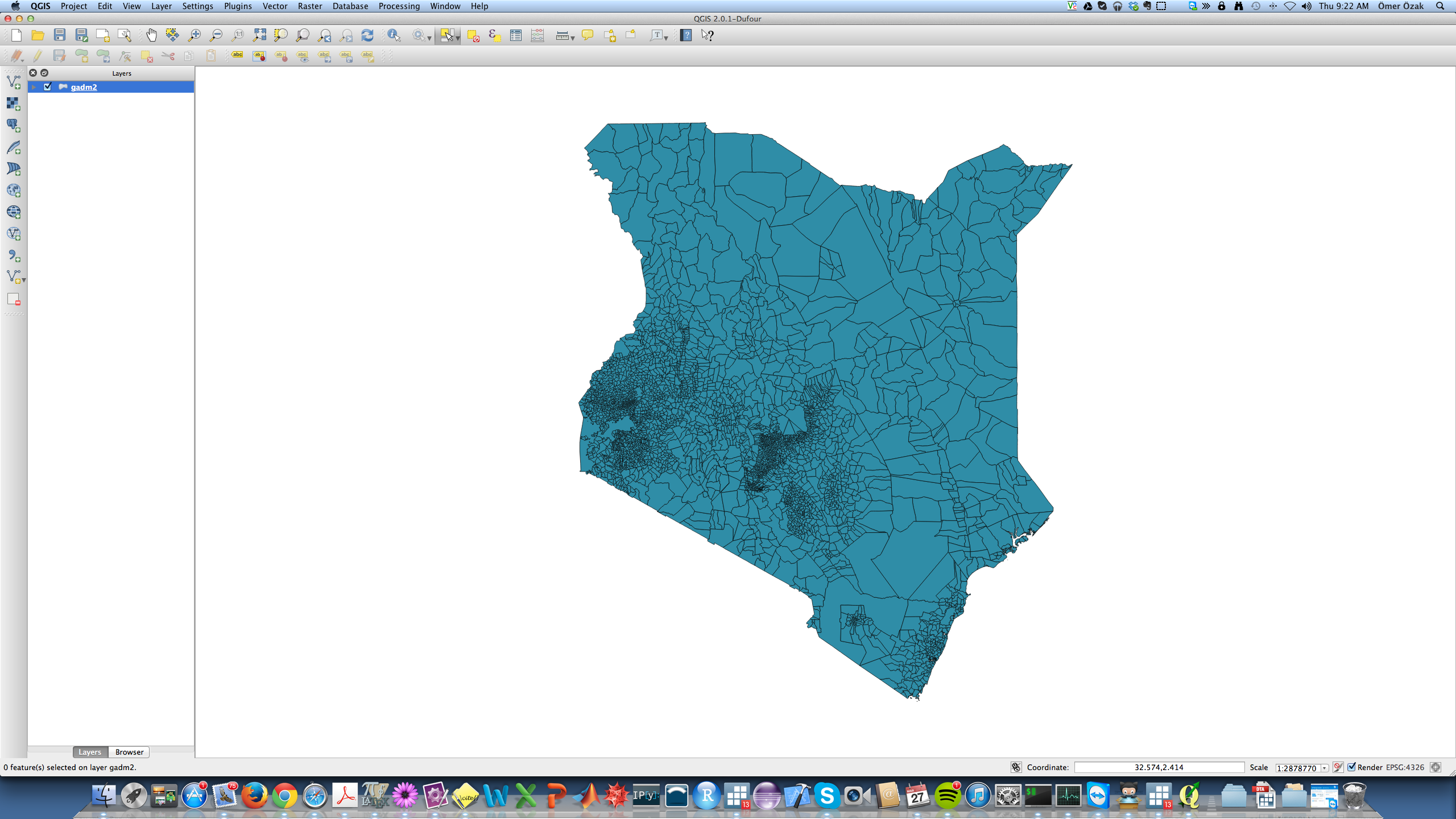
Let us zoom into these features by right-clicking on the name of the layer and choosing Zoom to Layer Extent. This shows the extent of Kenya alone.
Other important tools can be found in Layer -> Properties or by double-clicking on the layer's name
Exercise
- Load the complete GADM dataset.
- Select the regions of your country of origin, so that you will work only on these.
- Save the result to a new layer/shapefile called
your_country.shp
Vector Menu
The Vector menu has many tools that can be applied to vector layers. Let's use some of these to create new layers.
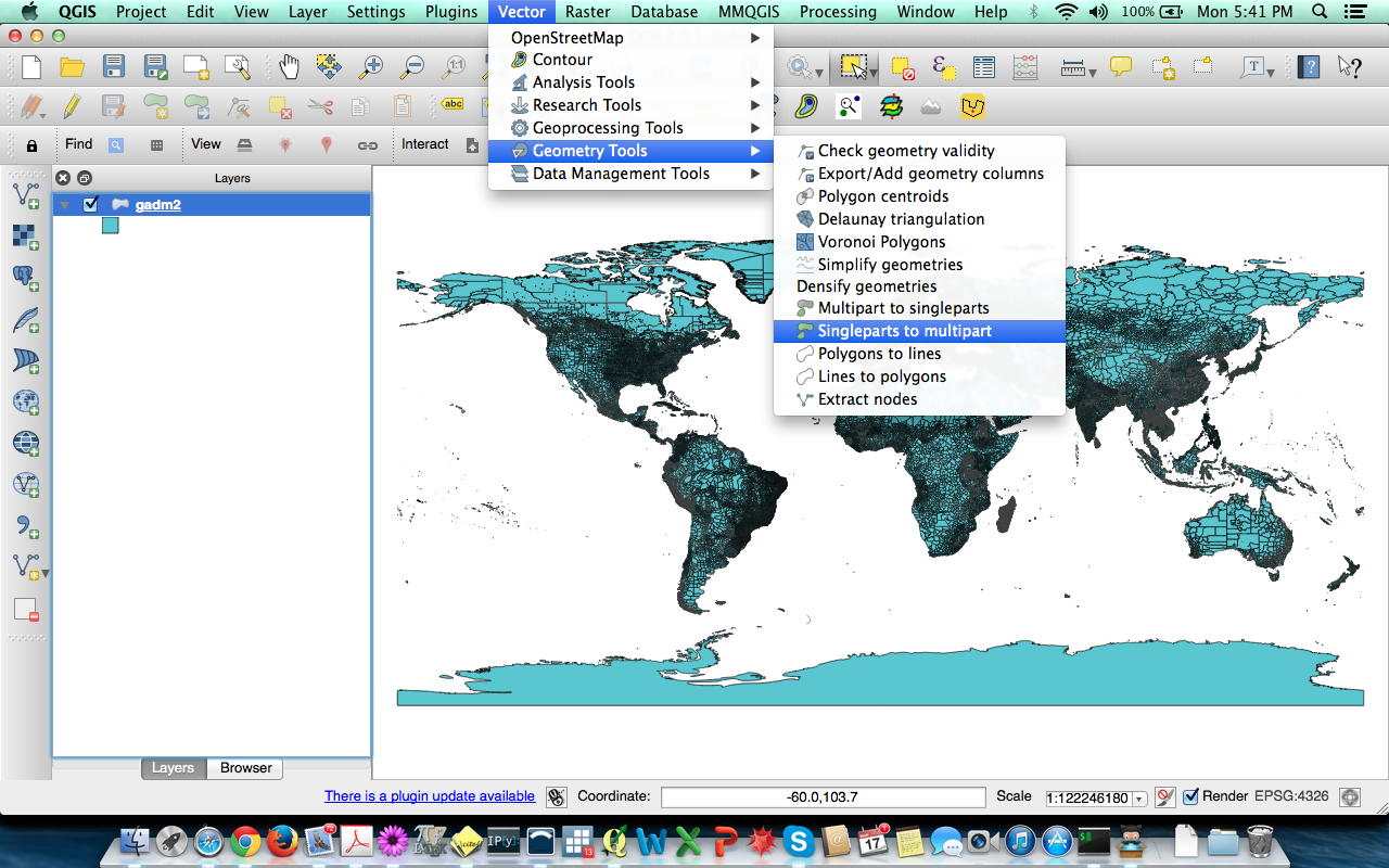
Using the Vector -> Geometry Tools -> Singlepart to Mutliparts we can generate a new layer and shape file where features are aggregated according to some characteristic. Let us use this tool to aggregate administrative level 2 features to the administrative level 0 (Country) level. Thus, each feature will be a country (administrative level 0) instead of the current administrative level 2.
Using the Vector -> Geometry Tools -> Mutliparts to singlepart we can generate a new layer and shape file where features are disaggregated.

Exercises
- Load the Populated Places data.
- Select the cities that belong to your country and create a new shape file with the selection named
your_country_places.shp. - Load the
your_country.shpfile you had created in the previous exercise and compute the centroid for each Adminitrative level 1 in your country and export the layer to the fileyour_country_centroids1.shp. Search for your place of birth among the most populated places. Where you born in a populated place? If not, identify the closest most populated place. To do so, use Google or Wikipedia to find the latitude and longitude of your place of birth. Using your mouse and the
coordinatewindow at the bottom
to search for your location of birth.
Better yet, using the Plugins->Manage and Install Plugins menu, install the ZoomToCoordinates plugin
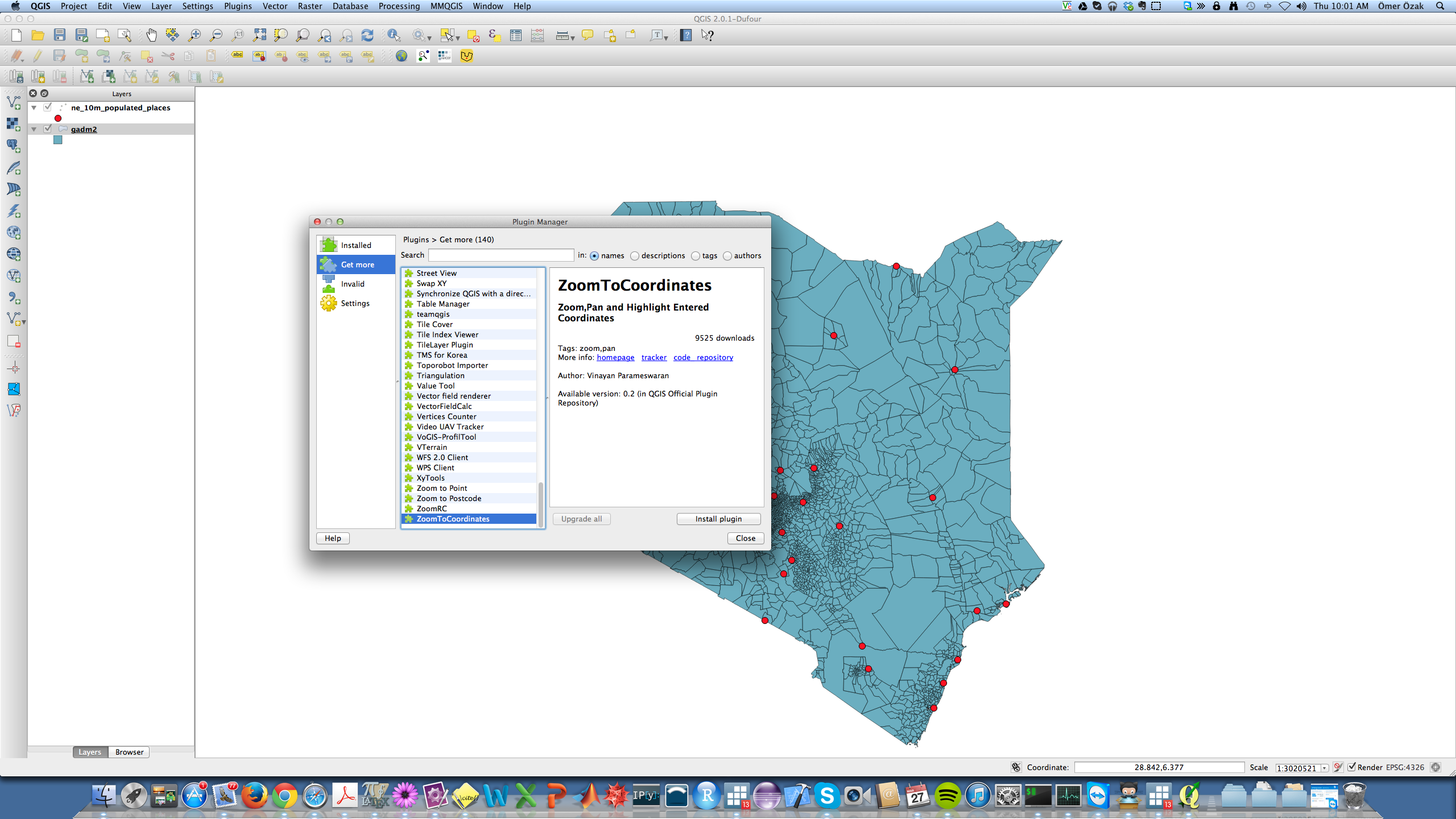
and use it to find your place of birth as shown below 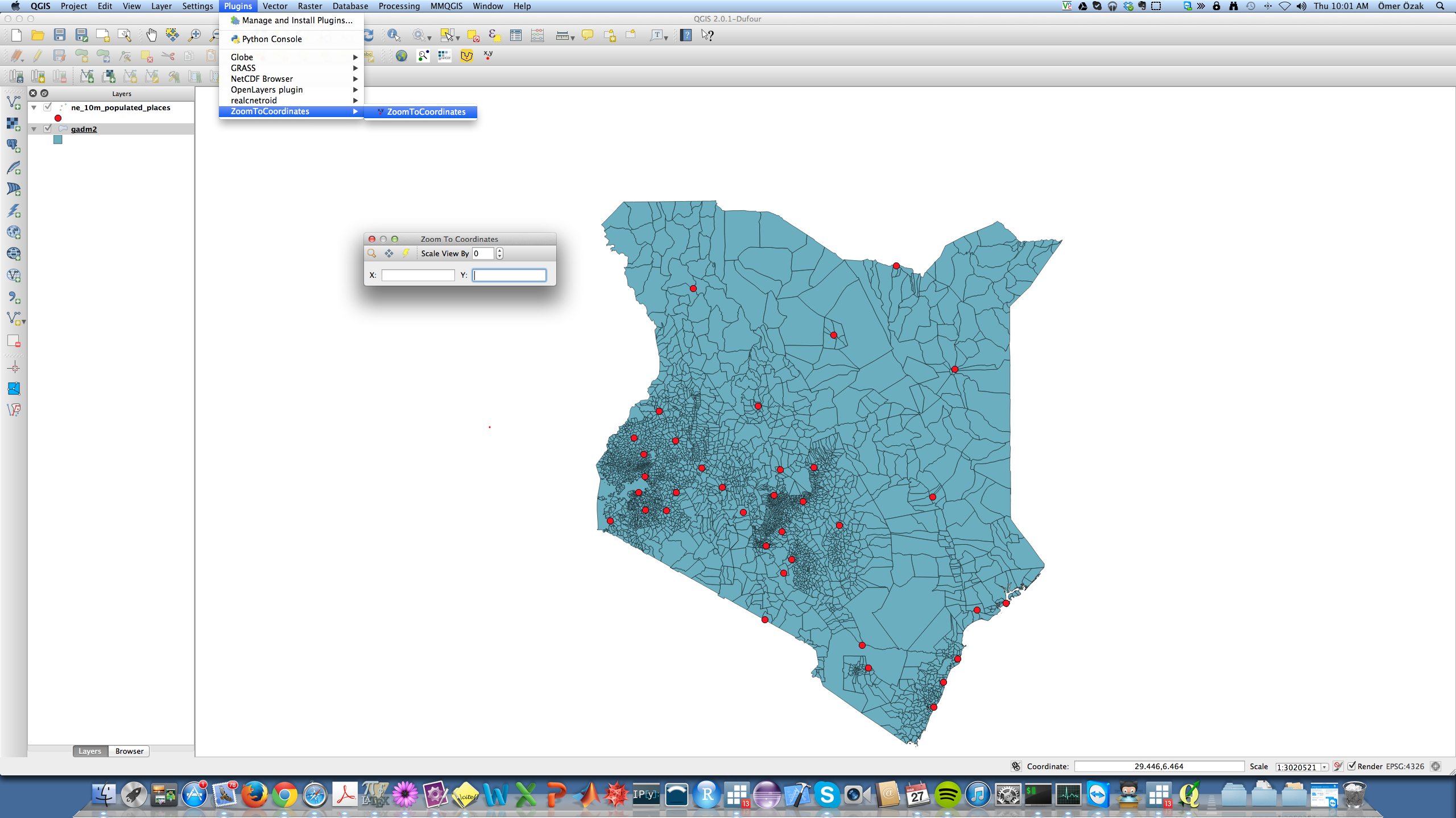
- Compute the distance between your place of birth and both the closest centroid and the closest most populated place. If needed find a Plugin that will do the job for you. I recommend installing among many
realcentroid,mmqgis,coordinate capture. - Generate the distance matrix among the most populated places
- Generate the distance matrix between most populated places and the centroids
Note
Make sure you can correctly identify the features. For example using ISO codes, ID numbers, etc. If the shape file does not have an ID identifier, it is best to create one, so that you can correctly identify the features. To do so, use the Field Calculator by double-clicking on the name of the layer, then choosing Fields. After that you need to select the pencil icon to enable editing mode.
Working with Rasters
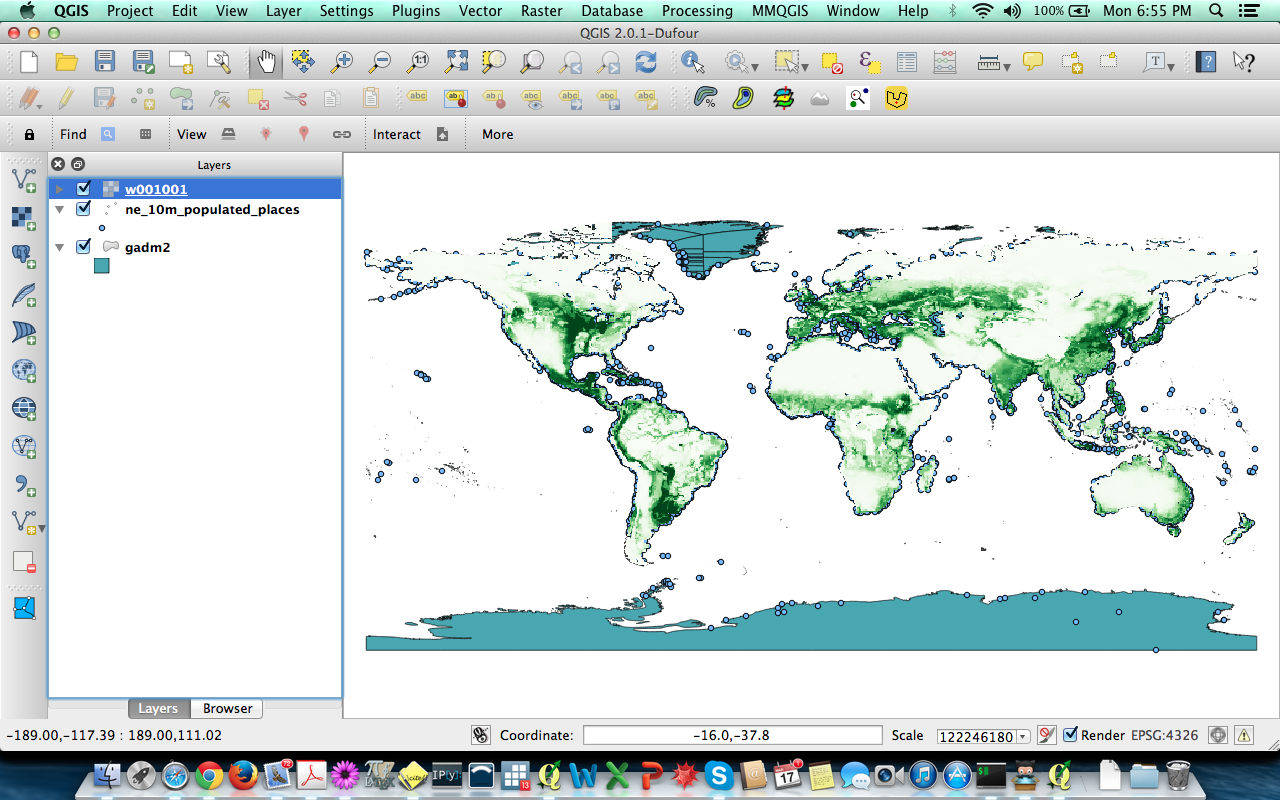
Let us load the Ramankutty raster using the add raster layer button in the toolbar.
Double-click on the name of the raster in order to change the coloring scheme.
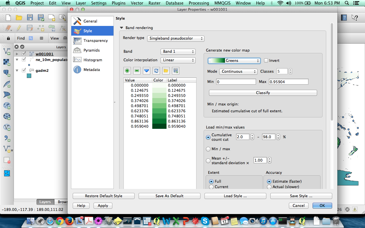
So it looks something like this
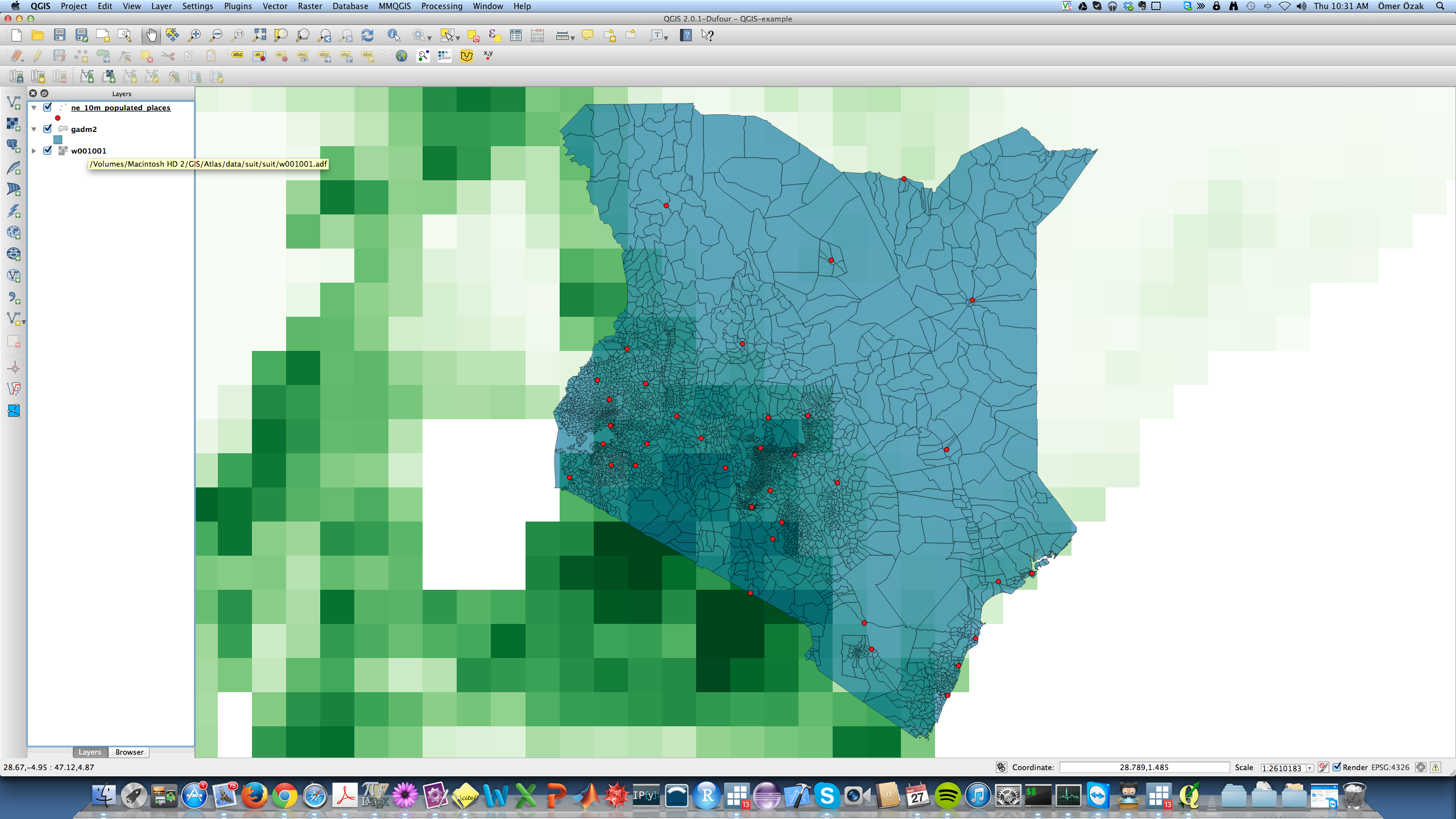
Load your your_country.shp and your_country_places.shp on top of the Ramankutty data. It might look something like this.
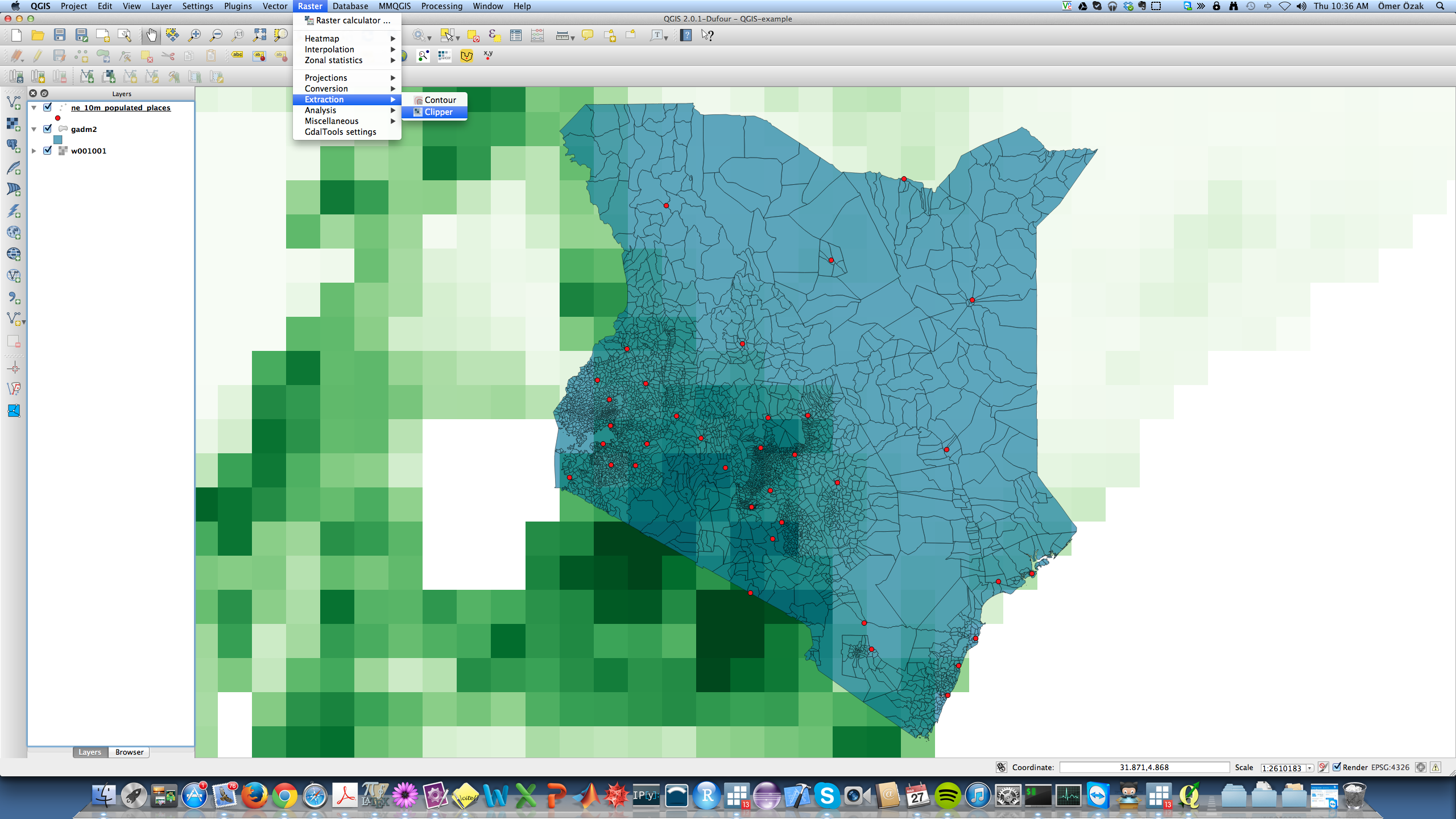
Since we do not want to work with all the Ramankutty data, but only with the data for our country, let us clip the part of the Ramankutty data that belongs to our country. To do this, use the Raster->Extraction->Clipper tool.
In the window that comes up, choose a name for the clipped raster suit_your_country and choose the save as GeoTiff option, so that your file is saved as in GeoTiff format. Then click on the Mask layer button, make sure your_country layer is chosen as the mask. If you want choose a different No data value. Then click ok.
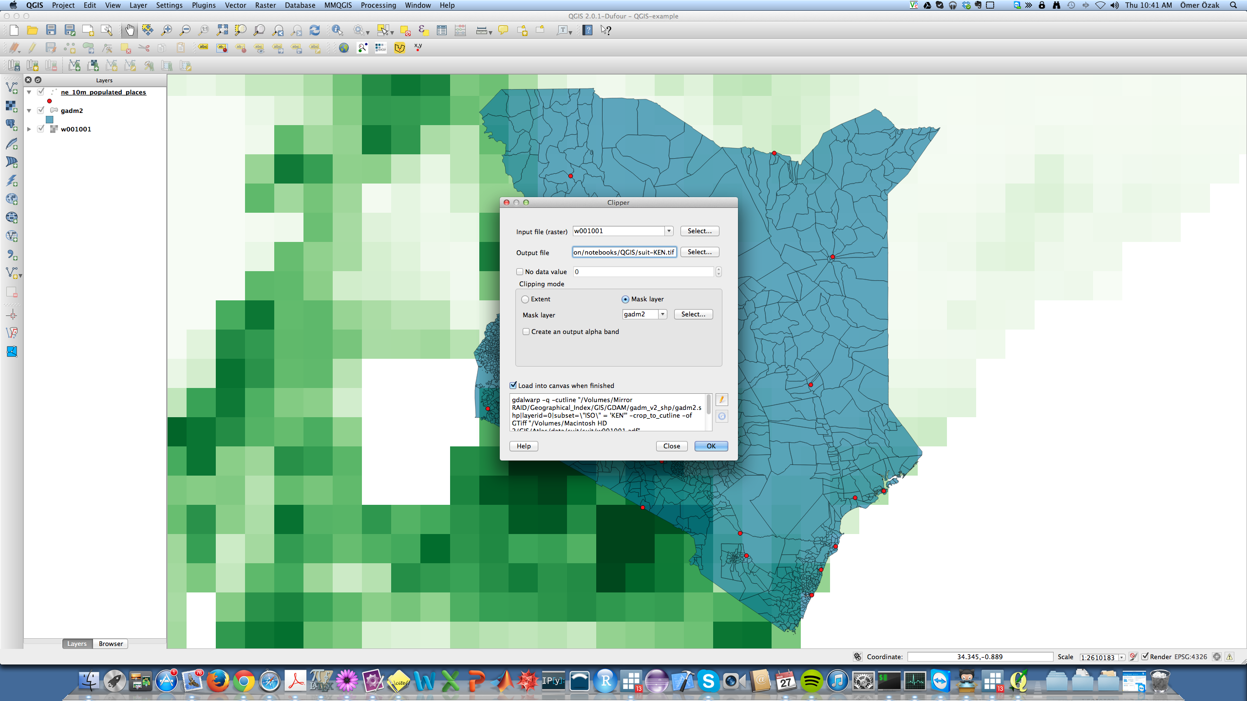
This will clip the Ramankutty data to the extent of your country of origin. Notice that in the big text box there is a command written, something like
gdalwarp -q -cutline "gadm2.shp|layerid=0|subset=\"ISO\" = 'KEN'" -crop_to_cutline -of GTiff "suit/w001001.adf" GitHub/CompEcon/notebooks/QGIS/suit-KEN.tif
This is a the command QGIS uses to create the clip. QGIS is actually calling GDAL to perform this operation. This command line will be very useful when you are planning to use Python or other scripting languages to perform an operation many times. You can do it by hand once and copy the command executed by QGIS and use it to create an iterable version...more on this later.
Note
You might have to assign a projection to the Suitability Raster. To do so, use the Raster->Projection->Assign Projection option in the menu.
The output should look like this
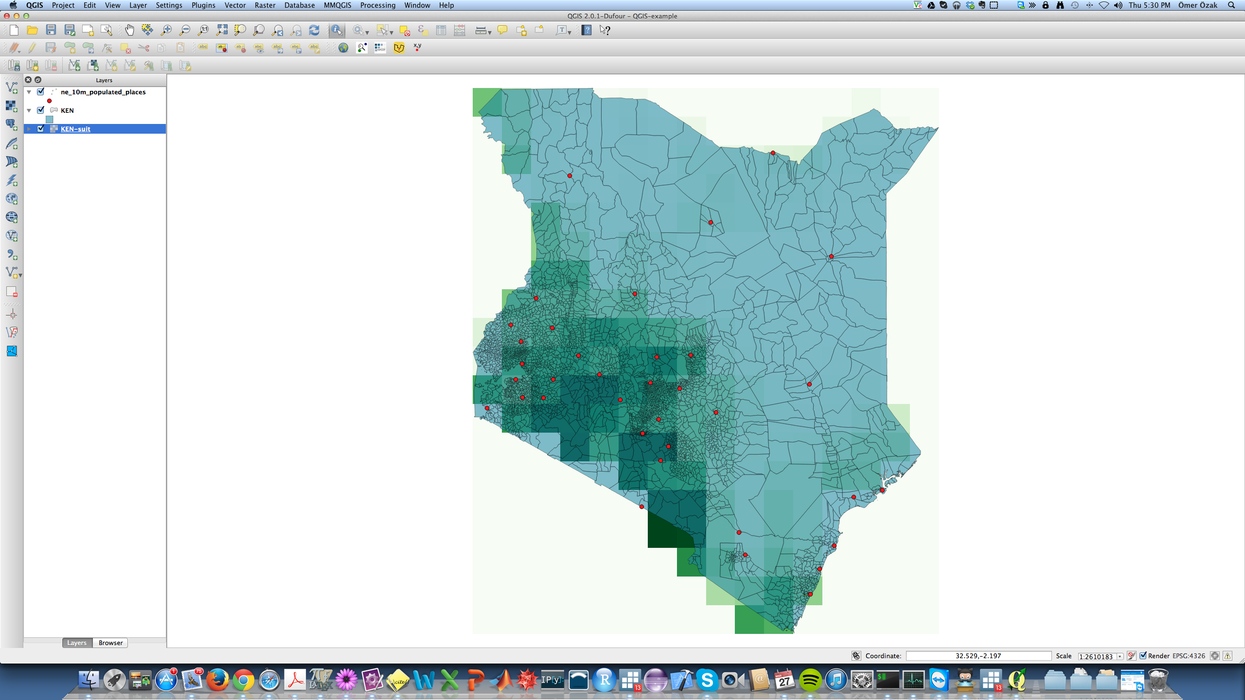
Notice that given the large size of the cells in the raster, the clipping tool creates a lot of measurement error. It might be better to decrease the size of cells an then clip, so that the clipping is less erroneous. Let's try setting the cell size to $5''$ instead of $0.5^o$. To do so, right-click on the raster name and select Save as. Then set the Resolution to $5''=1/12=0.08333$ for both Horizontal and Vertical.
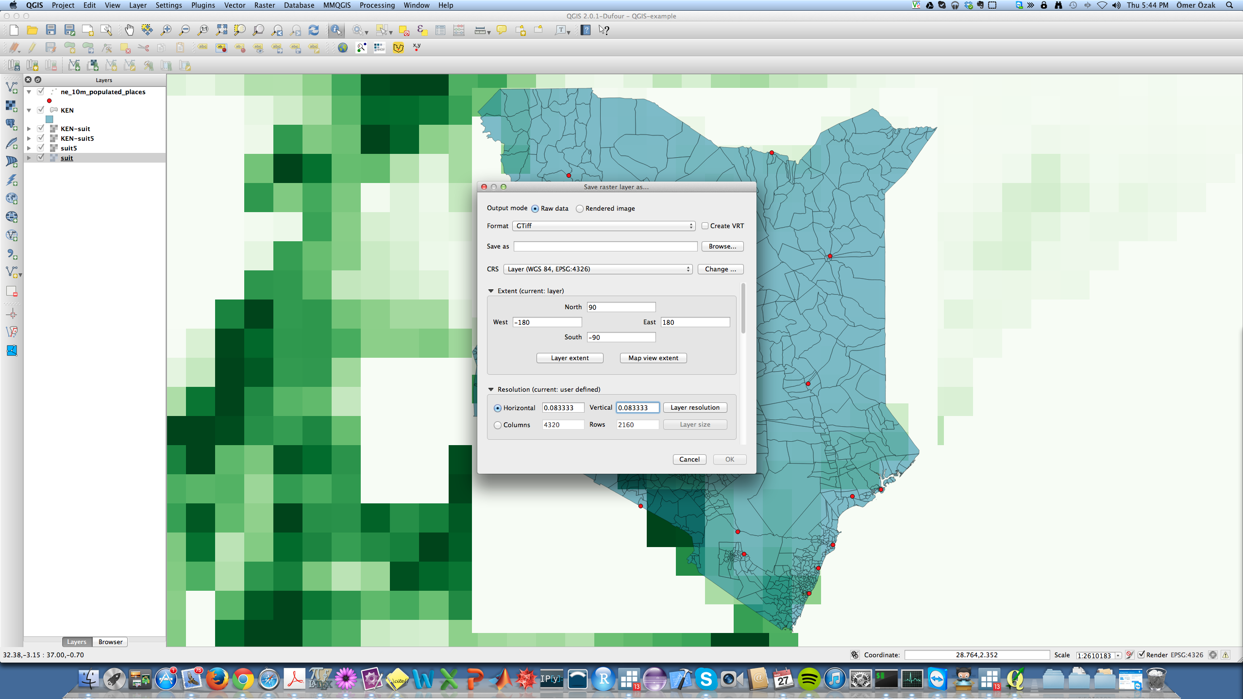
Now use the clip tool again. Much better! Obviously, the smaller the cell size, the more similar the clipped raster and the polygon will look like.
Note:
Care has to be taken when converting raster's cells size, since values have to be interpolated. QGIS seems to have taken away your choice for setting it. Luckily, GDAL can help out. You can use its tools to change the cells size, the projection, clip, etc. We will see some tools in another lecture.
Let us use this raster to assign the average suitability in each administrative region. But before doing so, we need to reproject both the raster and shape files to a format that ensures the areas are correctly take into account. One such projection is the equal area projection. Right click on the raster or shape and select save as.... Then in the CRS option choose Selected CRS and click on browse and choose the following CRS (or create it if not present by using the Settings->Custom CRS menu)
+proj=cea +lon_0=0 +lat_ts=0 +x_0=0 +y_0=0 +ellps=WGS84 +towgs84=0,0,0,0,0,0,0 +units=m +no_defs
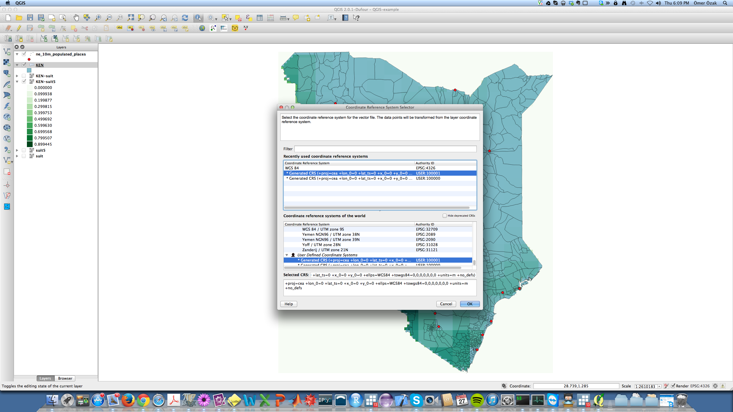
Now save the file adding the postfix cyl so that you know it is the cylindrical equal area rojected one. Now, select Raster->Zonal Statistics->Zonal Statistics.
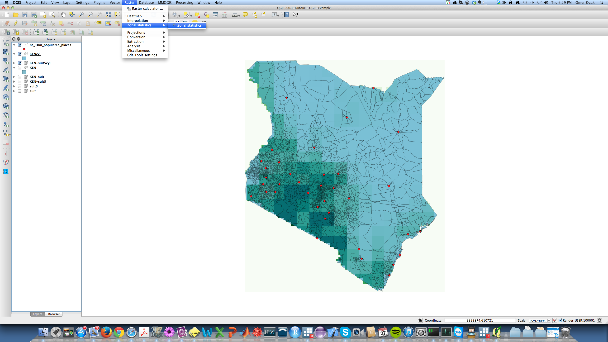
Select the cylindrical versions of the raster and shape files and suitcyl as the Output column prefix. Now, in the attribute table you will find three new columns with the prefix suitcyl that show the sum, count, and mean suitability in in each feature. If you repeat the analysis with the unprojected (non-cyl) versions of the raster and shape files, you will see that the results vary (sometimes significantly). Whenever you do this type of analysis, it is important to make sure you are using the correct projection for the analysis.
Other Raster Tools
In the Raster menu you will find other useful tools to work with rasters. Especially useful is the Raster Calculator, with which you can do computations on one or more rasters.
Exercises
- Import the Night Lights raster, convert it to a $5''$ raster, and clip it using your country's shapefile.
- Compute the average light in each region in your country.
- Generate a buffer of 100kms around each populated place and compute the average suitability and night lights for these buffers.
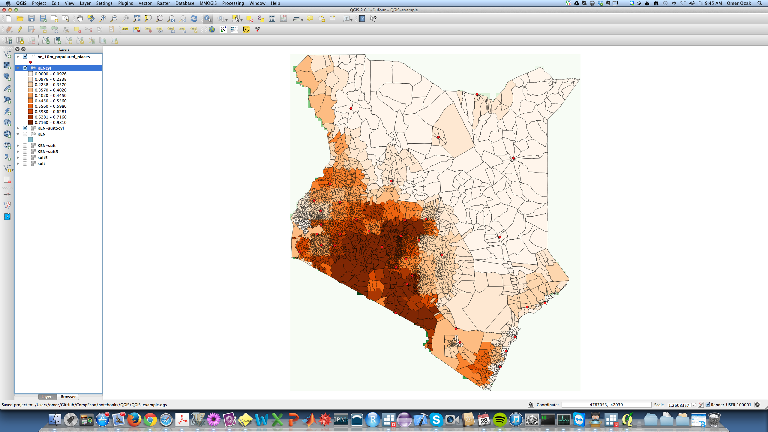
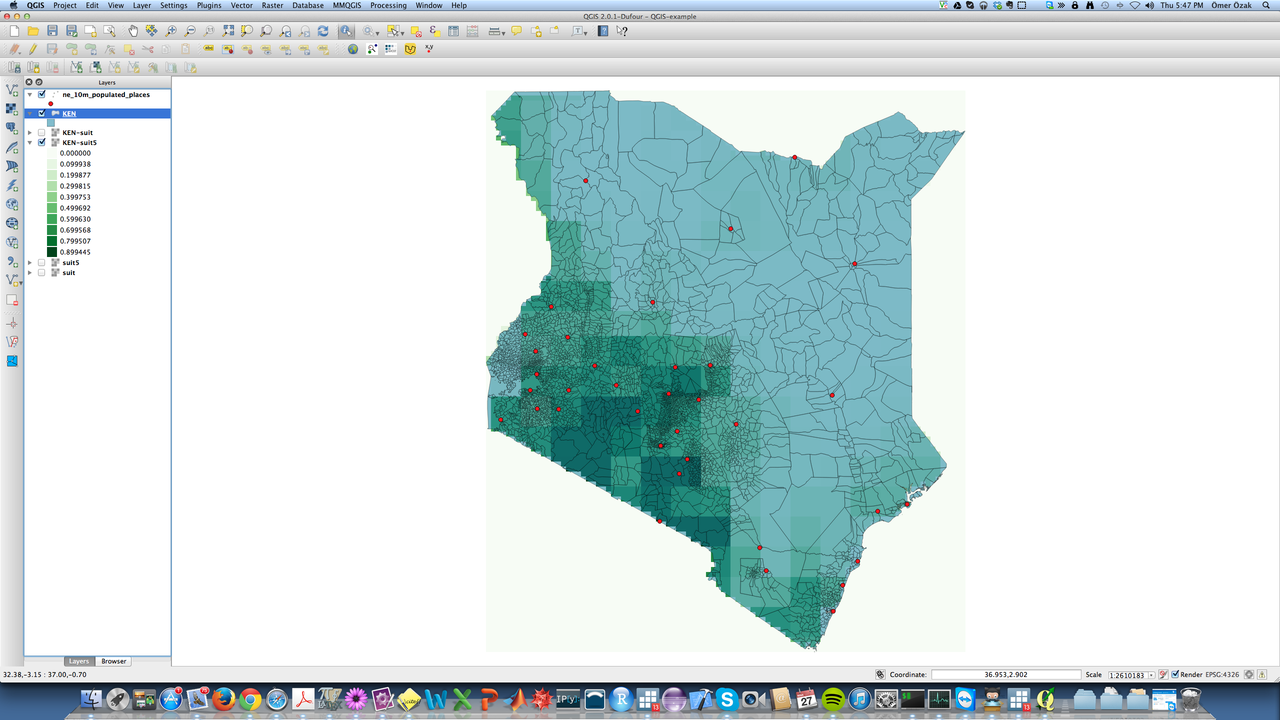
Adding Information and Using Colors
Now that you have the average agricultural suitability for each administrative region. Let's color code it so we can visually observe the regional differences. For this double-click on the your_country_cyl layer, which should open a new window in the style tab of the Layer->Properties menu.
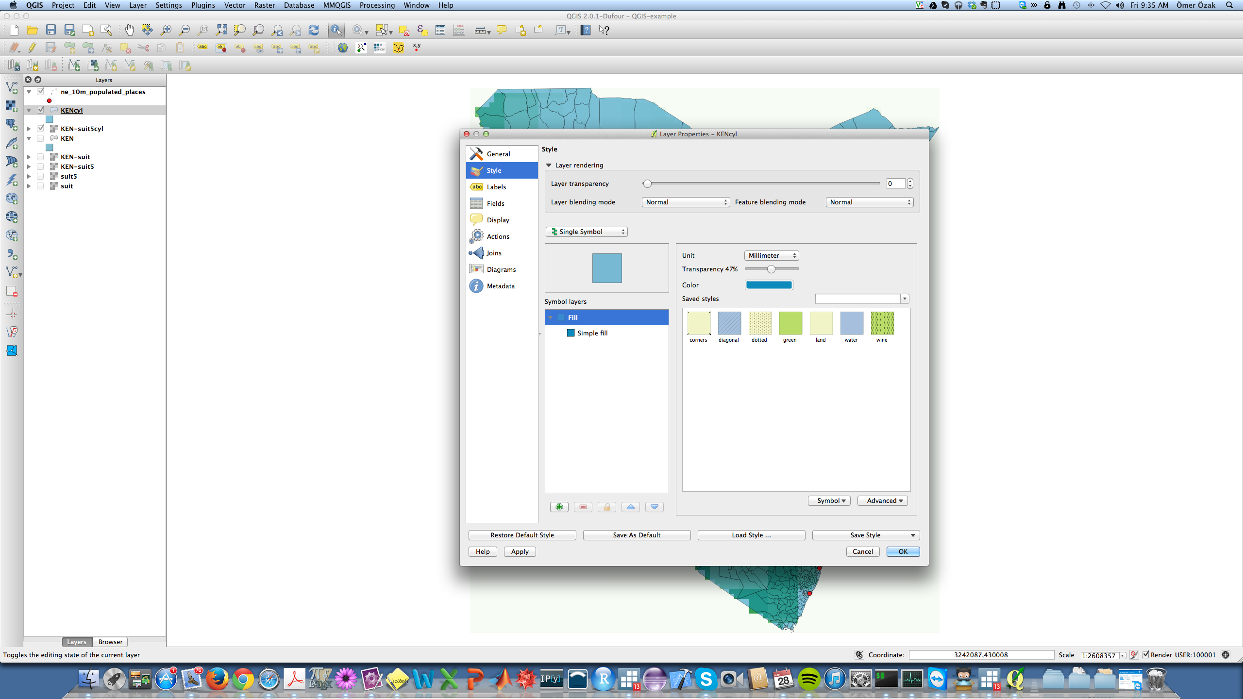
Now, click on Single Symbol and choose Graduated. This allows us to use colors to show the different values of a field/variable of interest.
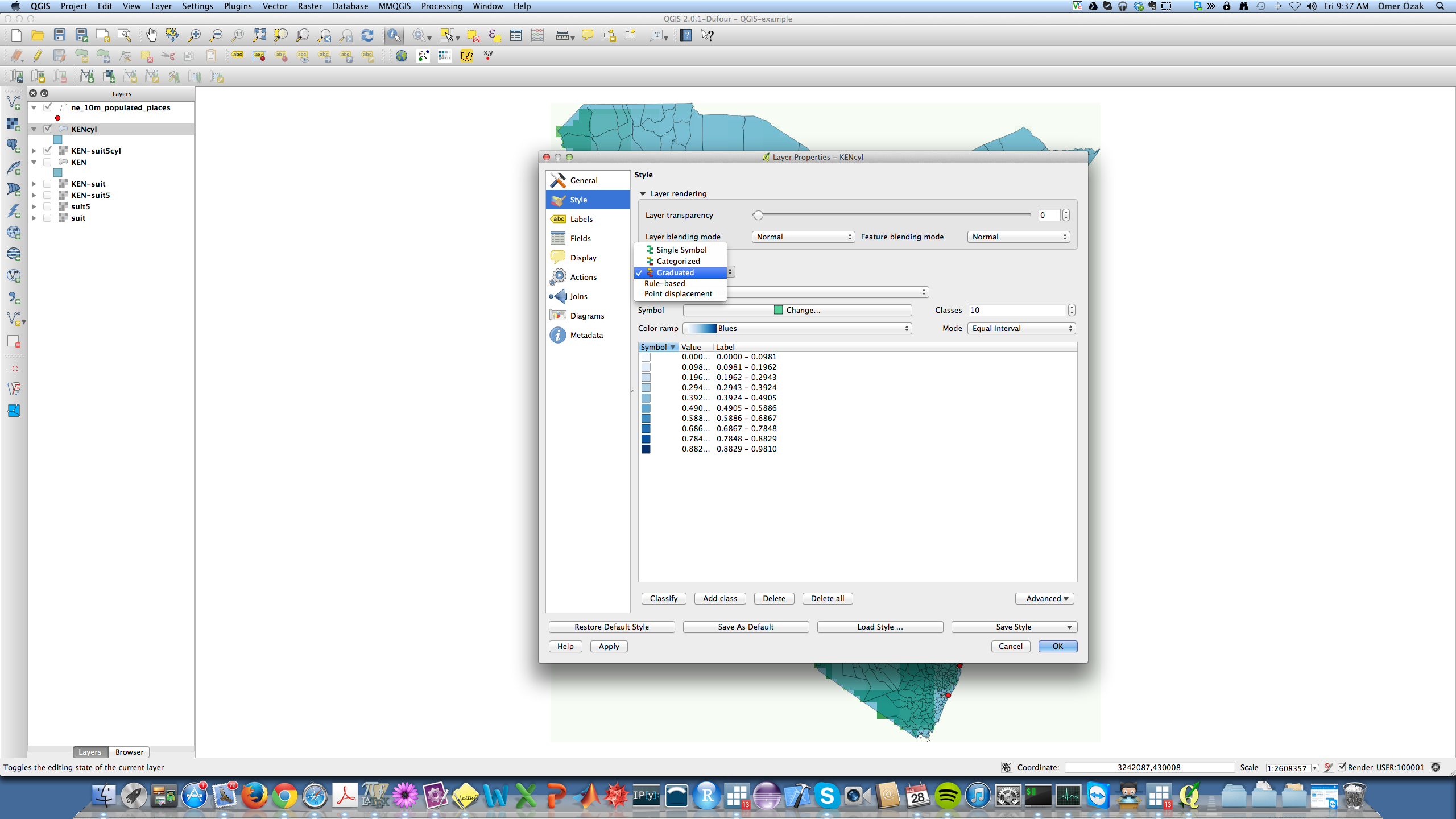
Next let us select the field of interest in the attribues table, namely, suitmean. To do so, click on column and choose the variable/field of interest, inthis case suitmean.
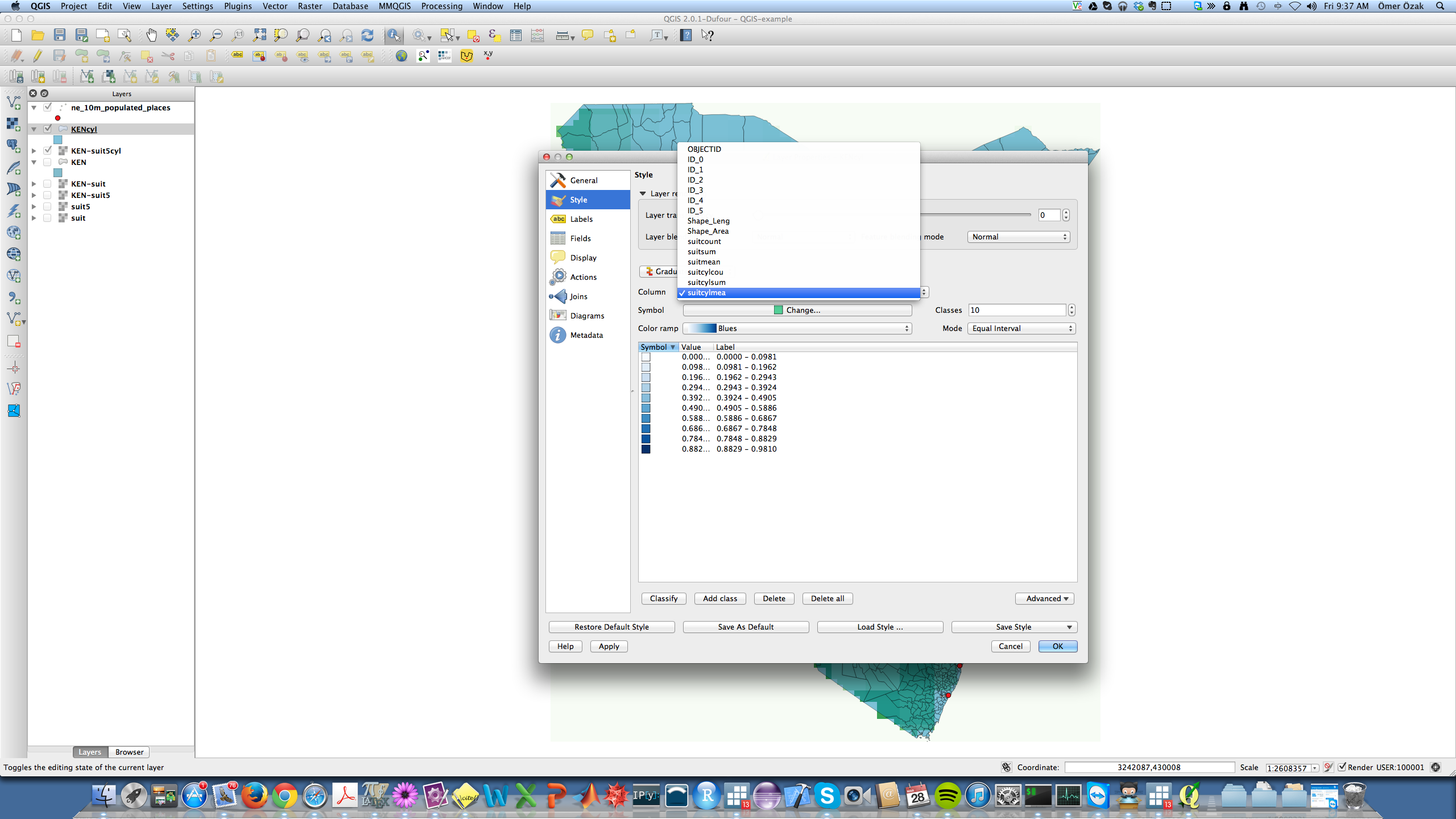
You can choose how many gradations to draw, e.g. increasing it from 5 to 10; change the color ramp, or the mode of creating the gradation. Try it out. You should get something like this